Visual Pathfinding with BFS, Dijkstra, and A*
Compare how BFS, Dijkstra, and A* explore a grid, calculate costs, and rebuild paths using queues, priority queues, and heuristics.

Pathfinding is not about finding any route. It is about finding a route that respects the map and optimizes the right measure: steps, cost, time, risk, or a combination of them.
BFS, Dijkstra, and A* share most of their mechanism. All three keep a frontier of pending states and a record for rebuilding the path. What changes is which state leaves the frontier first.
Before choosing an algorithm, define the moves, the costs, and the guarantee that makes a route correct.
01. Before the algorithm: turn the map into a graph
In a grid, every traversable cell is a vertex and every allowed move is an edge. With four-direction movement, a cell can connect up, down, left, and right. Adding diagonals changes the edges, their cost, and the valid heuristic.
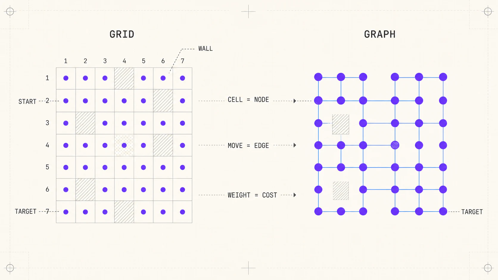 Visual conversion of a grid into graph nodes and edges
type Point = { x: number; y: number };

type Cell = {
  walkable: boolean;
  weight: number;
};

const directions = [
  { x: 1, y: 0 },
  { x: -1, y: 0 },
  { x: 0, y: 1 },
  { x: 0, y: -1 },
];

function key({ x, y }: Point) {
  return `${x},${y}`;
}

function neighbors(point: Point, grid: Cell[][]) {
  return directions
    .map(({ x, y }) => ({ x: point.x + x, y: point.y + y }))
    .filter((next) => grid[next.y]?.[next.x]?.walkable);
}
The map contract must answer four questions:
- Which moves are allowed?
- Does cost belong to the destination cell or to the edge?
- Can a diagonal move cut through a blocked corner?
- Are all weights non-negative?
In a grid with V cells and four neighbors, there is at most a constant number of edges per cell, so E grows like V. It is still useful to write O(V + E) because the same reasoning applies to graphs that are not grids.
02. One frontier, three priority rules
All three algorithms discover neighbors, record the best known parent, and repeat until they extract the goal or exhaust the frontier.
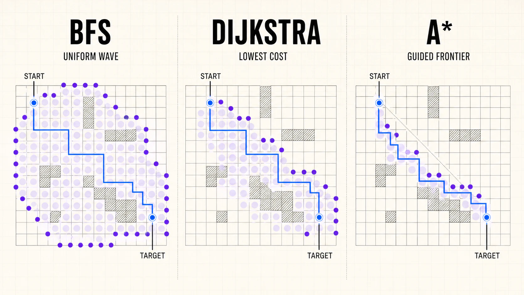 Comparison of BFS, Dijkstra, and A* frontiers on the same map
| Algorithm | Frontier | Priority | Guarantee |
|---|---|---|---|
| BFS | FIFO queue | discovery order | fewest edges when every step has equal cost |
| Dijkstra | min-heap | g(n) | lowest cost with non-negative weights |
| A* | min-heap | g(n) + h(n) | lowest cost when the heuristic is admissible |
A* notation separates what is known from what is estimated:
f(n) = g(n) + h(n)

g(n): actual cost from the start
h(n): estimated remaining cost to the goal
BFS traverses in O(V + E). Dijkstra with a binary min-heap commonly costs O((V + E) log V). A* keeps that general worst case, although a good heuristic can greatly reduce the number of expanded states.
That last distinction matters in a lab: theoretical complexity does not change, but the visible frontier can go from covering almost the entire map to forming a corridor toward the goal.
03. BFS: the right choice for uniform cost
BFS explores in layers. Marking a cell when it is enqueued prevents duplicates, and a head index lets the array act as a queue without the repeated shifting cost of shift().
function bfs(start: Point, goal: Point, grid: Cell[][]) {
  const queue = [start];
  const parent = new Map<string, Point | null>([[key(start), null]]);

  for (let head = 0; head < queue.length; head += 1) {
    const current = queue[head];
    if (key(current) === key(goal)) break;

    for (const next of neighbors(current, grid)) {
      const nextKey = key(next);
      if (parent.has(nextKey)) continue;

      parent.set(nextKey, current);
      queue.push(next);
    }
  }

  return parent;
}
BFS guarantees the route with the fewest moves when every move has the same cost. If grass, water, and roads have different weights, counting steps no longer represents the objective and you need Dijkstra or A*.
Its visual pattern is a wave. That broad expansion is not a flaw: it is the price of having no information that favors one direction.
04. Dijkstra and A*: the same engine, a different priority
Dijkstra and A* use the same relaxation rule: when a new route reaches a neighbor with lower cost, they update its distance, parent, and frontier entry. The difference is the priority.
type FrontierItem = {
  point: Point;
  cost: number;
  priority: number;
};

function weightedSearch(
  start: Point,
  goal: Point,
  grid: Cell[][],
  heuristic: (point: Point, goal: Point) => number,
) {
  const frontier = new MinPriorityQueue<FrontierItem>(
    (item) => item.priority,
  );
  frontier.push({ point: start, cost: 0, priority: 0 });

  const cost = new Map<string, number>([[key(start), 0]]);
  const parent = new Map<string, Point | null>([[key(start), null]]);

  while (!frontier.isEmpty()) {
    const current = frontier.pop();
    if (current.cost !== cost.get(key(current.point))) continue;
    if (key(current.point) === key(goal)) break;

    for (const next of neighbors(current.point, grid)) {
      const nextCost = current.cost + grid[next.y][next.x].weight;
      const knownCost = cost.get(key(next));

      if (knownCost === undefined || nextCost < knownCost) {
        cost.set(key(next), nextCost);
        parent.set(key(next), current.point);
        frontier.push({
          point: next,
          cost: nextCost,
          priority: nextCost + heuristic(next, goal),
        });
      }
    }
  }

  return { parent, cost };
}
The example assumes a MinPriorityQueue implemented with a binary heap. Calling sort() on every iteration is convenient for a tiny demonstration, but it hides the real cost and is not representative of a production implementation.
With heuristic = () => 0, the engine is Dijkstra. With a valid estimate toward the goal, it is A*. The stale-entry check prevents expanding an old priority after a better route has been found.
The goal should stop the search when it leaves the priority queue as the best pending state, not when it is first discovered.
05. Honest heuristics and reconstructable routes
An admissible heuristic never overestimates the remaining cost. In a weighted grid it should be scaled by the lowest possible step cost; otherwise a geometric distance may promise more or less than the rules allow.
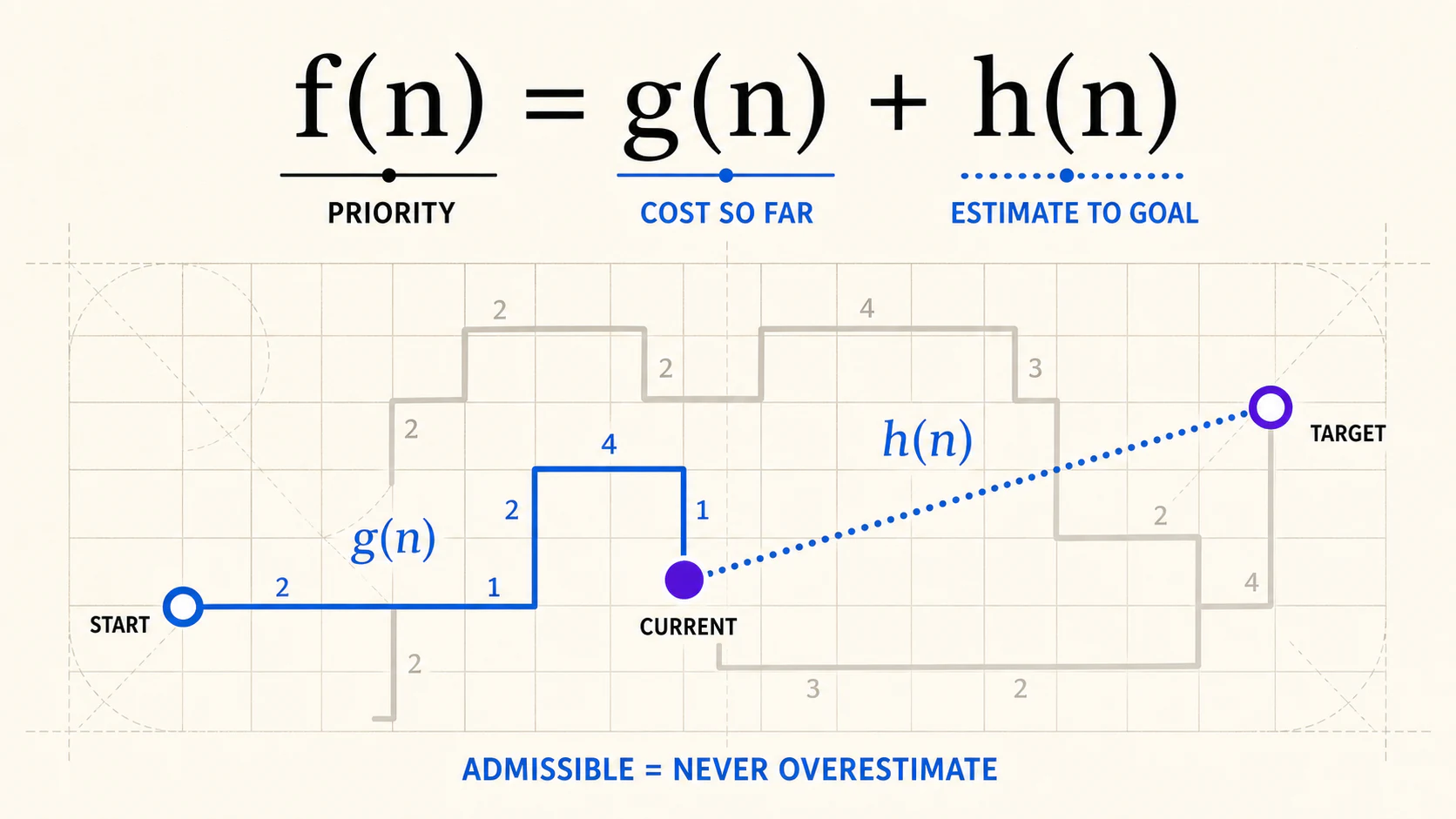 Visual decomposition of A* priority into accumulated cost and estimate
| Movement | Starting heuristic | Condition |
|---|---|---|
| four directions | Manhattan | orthogonal costs and no diagonals |
| eight directions | Octile or Chebyshev | depends on the assigned diagonal cost |
| continuous space | Euclidean | straight-line distance is a valid lower bound |
| no safe estimate | zero | A* becomes Dijkstra |
The heuristic changes exploration order, not the actual cost stored in g(n). If it overestimates, A* can become more aggressive but loses its optimality guarantee.
The final route is rebuilt by following parents back from the goal. First verify that the goal was reached:
function reconstructPath(
  parent: Map<string, Point | null>,
  start: Point,
  goal: Point,
) {
  if (!parent.has(key(goal))) return [];

  const path: Point[] = [];
  let current: Point | null = goal;

  while (current) {
    path.push(current);
    if (key(current) === key(start)) break;
    current = parent.get(key(current)) ?? null;
  }

  return path.reverse();
}
Visually separating visited, frontier, and final route avoids a common confusion: exploring a cell does not mean that the cell belongs to the chosen path.
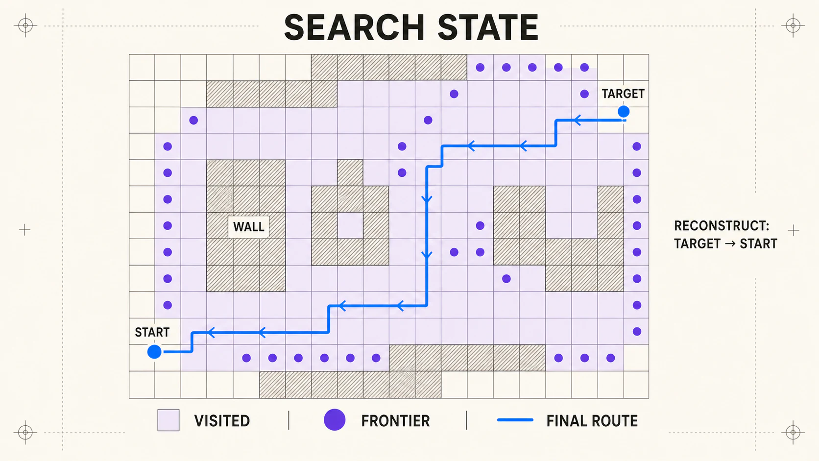 Search states and route reconstruction from the goal back to the start
06. How to choose and what the experiment should measure
| Situation | Starting choice |
|---|---|
| every move has equal cost | BFS |
| non-negative weights and no useful heuristic | Dijkstra |
| known goal and admissible heuristic | A* |
| negative weights | another algorithm; these three do not apply directly |
| continuously changing map | recompute or use incremental planning |
The lab should run all three algorithms on the same map and display at least:
- expanded nodes;
- maximum frontier size;
- final route cost and length;
- computation time separated from animation time;
- a no-route state when the goal is unreachable.
It should also prevent unfair comparisons. BFS cannot compete on cost if it ignores weights, and A* should not receive a heuristic that conflicts with movement rules. For maps that change in small regions, incremental algorithms such as LPA* or D* Lite can avoid recomputing from scratch.
The practical decision is simple: BFS minimizes uniform steps; Dijkstra minimizes actual cost; A* searches for the same optimum while using additional information to guide the frontier. The map defines the problem, the priority defines the exploration, and the parent record turns that exploration into a route.