Search Algorithms: Collections, Graphs, and Pathfinding with BFS, Dijkstra, and A*
A practical guide for separating collection search from graph search, and choosing between Linear, Binary, Hash Map, BFS, DFS, Dijkstra, and A*.

“Search” can mean finding a record in an array, checking a key in an index, or discovering a route between states. The word is the same; the structure, cost, and guarantee are completely different.
Binary Search does not compete with A*. The first reduces a sorted collection. The second explores a graph using costs and an estimate toward a goal. Before choosing an algorithm, identify the problem's shape.
First decide where you are searching; then decide which guarantee you need.
01. Three shapes of search
Most problems in this guide fall into three families:
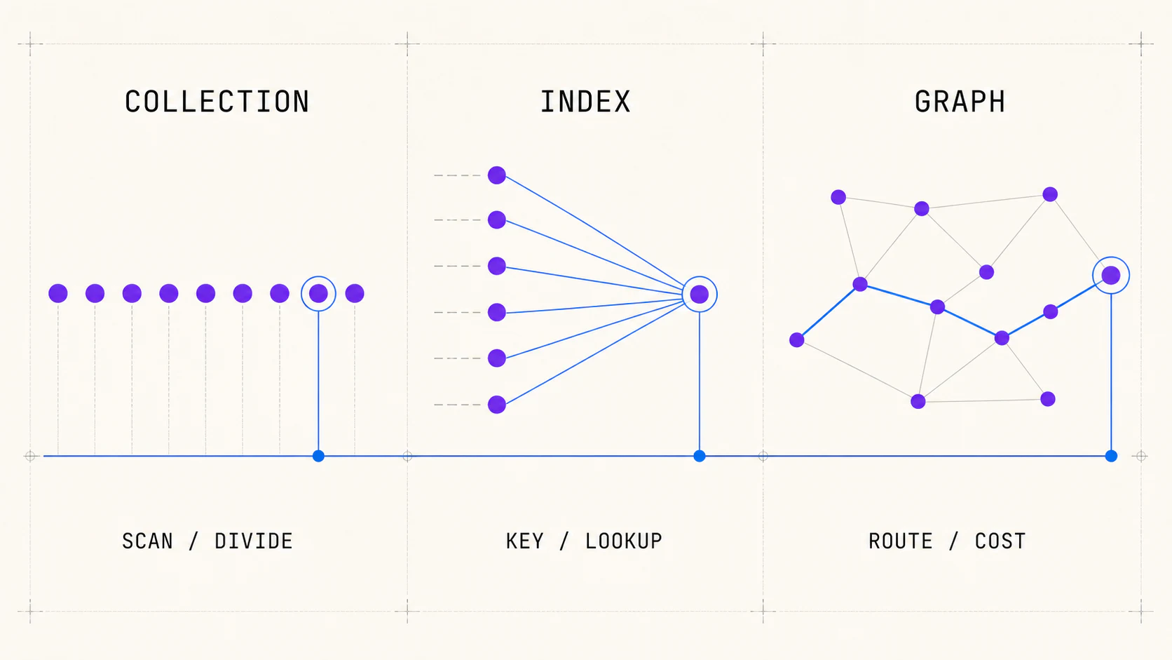 Three search universes: collection, index, and graph
| Problem shape | Question | Starting options |
|---|---|---|
| collection | Where is this item? | Linear or Binary Search |
| key index | Does the record with this id, email, or slug exist? | Map or Set |
| graph of states or relationships | Can I reach it, and what is the best route? | BFS, DFS, Dijkstra, or A* |
Inside a collection, existing order and query count matter. Inside a graph, weights, the goal, and the required guarantee matter: reach, traverse, minimize steps, or minimize cost.
A useful rule is to measure total work, not only one lookup:
total cost = preparation + query count × cost per querySorting or building an index can cost more than a linear scan. It pays off when you reuse that preparation or when order enables other operations such as ranges and bounds.
02. Collections: scan, divide, or index
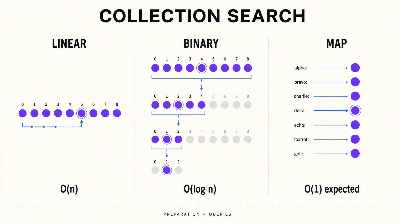 Visual comparison of Linear Search, Binary Search, and Map
Linear Search
It scans until it finds a match or reaches the end. It costs O(n) in the worst case, uses O(1) additional space, and needs no preparation. For a small collection or an isolated query, it is often the cheapest decision.
Binary Search
It compares against the middle and discards the impossible half. Every step reduces the universe, so it costs O(log n). Its precondition is order, and that order must use the same criterion as the search.
function binarySearch(values: number[], target: number) {
  let low = 0;
  let high = values.length - 1;

  while (low <= high) {
    const middle = low + Math.floor((high - low) / 2);
    const value = values[middle];

    if (value === target) return middle;
    if (value < target) low = middle + 1;
    else high = middle - 1;
  }

  return -1;
}
Binary Search also supports lowerBound and upperBound: finding the first value not smaller than a target or the first value greater than it. Order provides something a hash cannot provide directly.
Map and Set
An index transforms repeated queries. Building it costs O(n) and O(n) memory, but looking up a key commonly costs expected O(1):
const usersByEmail = new Map(users.map((user) => [user.email, user]));

const user = usersByEmail.get("ada@example.com");
const exists = usersByEmail.has("ada@example.com");
The tradeoff is clear: Map serves key equality; Binary Search preserves order and enables ranges; Linear Search prepares nothing and accepts any condition.
03. Unweighted graphs: the frontier decides the traversal
A graph represents connected nodes: cities, screens, dependencies, cells, states, or people. With an adjacency list, BFS and DFS run in O(V + E) because they visit every vertex and edge a constant number of times.
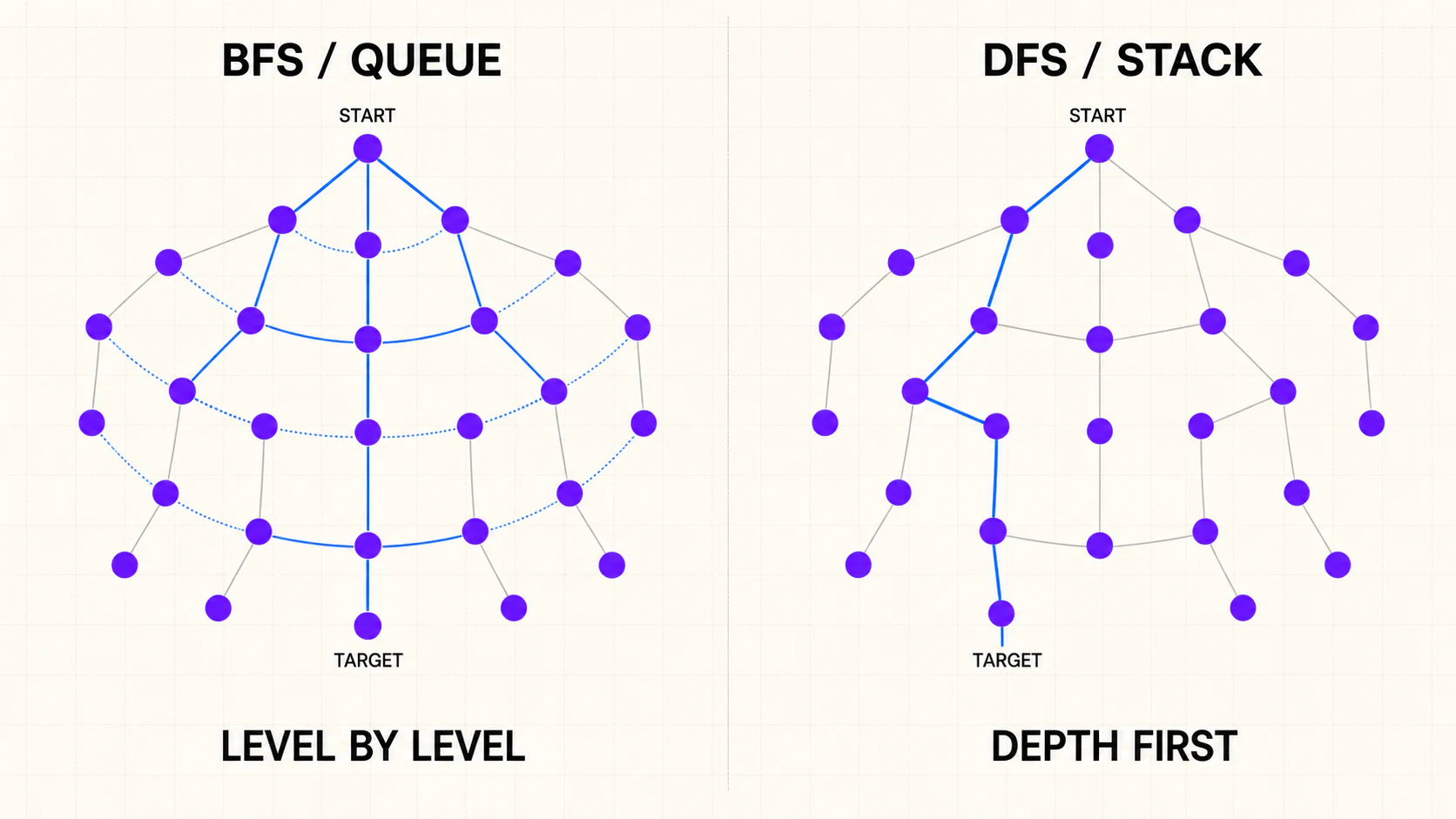 Comparison of the exploration frontier in BFS and DFS
The main difference is the frontier:
| Method | Frontier | What it prioritizes | Useful guarantee |
|---|---|---|---|
| BFS | FIFO queue | nodes closer in steps | path with the fewest edges when unweighted |
| DFS | LIFO stack or recursion | one branch to its depth | reachability, traversal, and backtracking |
BFS stores complete levels and may use more memory in wide graphs. DFS commonly keeps one active route, but it can go very deep and does not guarantee the shortest path.
A BFS implementation needs to record parents—not only visited nodes—if you want to reconstruct the route:
function bfs(graph: Map<string, string[]>, start: string) {
  const queue = [start];
  const parent = new Map<string, string | null>([[start, null]]);

  for (let head = 0; head < queue.length; head += 1) {
    const node = queue[head];

    for (const neighbor of graph.get(node) ?? []) {
      if (parent.has(neighbor)) continue;
      parent.set(neighbor, node);
      queue.push(neighbor);
    }
  }

  return parent;
}
Using a head index avoids the repeated shifting that shift() could cause in a large queue.
04. Cost-aware paths: Dijkstra and A*
When edges have weights, fewer steps no longer means lower cost. A three-segment route can be cheaper than a two-segment route.
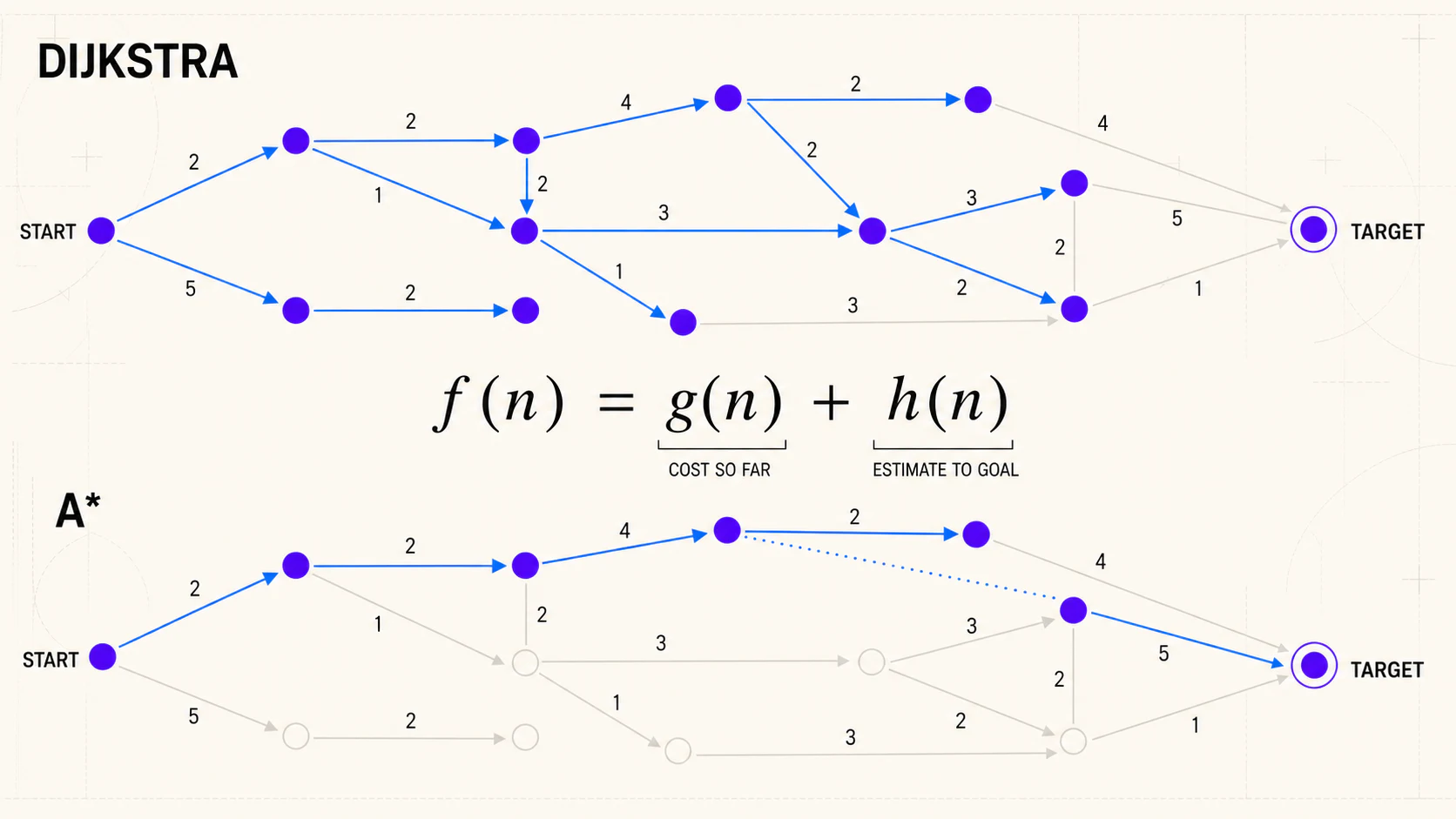 Visual comparison of Dijkstra and A* using accumulated cost and a heuristic
Dijkstra always expands the pending node with the lowest accumulated cost. With an adjacency list and binary priority queue, its common cost is O((V + E) log V). It requires non-negative weights: a negative edge can invalidate a distance that already looked final.
A* adds an estimate toward a goal:
f(n) = g(n) + h(n)

g(n): accumulated cost from the start
h(n): estimated remaining cost to the goal
If h(n) = 0, A* behaves like Dijkstra. A useful heuristic can avoid large regions of the graph; a weak heuristic explores more. To preserve optimality, the estimate must not overestimate the remaining cost—and a consistent heuristic is commonly used.
| Situation | Method | Reason |
|---|---|---|
| every edge has equal cost | BFS | minimizes steps without a priority queue |
| non-negative weights, no spatial guidance | Dijkstra | minimizes accumulated cost |
| known goal and admissible heuristic | A* | prioritizes promising states |
| negative weights exist | another method such as Bellman–Ford | standard Dijkstra and A* do not apply |
A* is not “fast Dijkstra” by definition. The gain depends on the quality and cost of h(n), graph representation, and how many states it avoids exploring.
05. Decision table and mistakes that invalidate the answer
| Need | Starting method | Preparation | Query or traversal |
|---|---|---|---|
| one match in unordered data | Linear Search | O(1) | O(n) |
| lookup and ranges in sorted data | Binary Search | existing order or O(n log n) | O(log n) |
| many exact-key queries | Map / Set | O(n) | expected O(1) |
| fewest steps in an unweighted graph | BFS | O(V + E) representation | O(V + E) |
| deep traversal or backtracking | DFS | O(V + E) representation | O(V + E) |
| lowest cost with non-negative weights | Dijkstra | priority queue | O((V + E) log V) |
| lowest cost with a goal and heuristic | A* | priority queue + h(n) | heuristic-dependent; broad worst case |
The important mistakes are not syntactic; they break preconditions:
- Running Binary Search on data that does not respect the comparator's order.
- Building a
Mapfor one query and hiding construction and memory cost. - Using DFS while expecting the path with the fewest steps.
- Using BFS when edge costs differ.
- Running Dijkstra with negative weights.
- Using A* with an overestimating heuristic while still expecting optimality.
06. Selection checklist
Before writing code, answer:
- Are you looking for an item, an exact key, or a route?
- Is the data already sorted, and do you need ranges?
- How many queries will reuse the preparation?
- Does the graph have weights, and can they be negative?
- Do you need to reach, traverse, minimize steps, or minimize cost?
- Is there a concrete goal and a defensible heuristic?
- Must you reconstruct the route, not only know that it exists?
Start with the simplest structure that supports the guarantee. Linear Search is correct when preparation costs too much; Binary Search when order matters; Map when a key is queried repeatedly; BFS and DFS when relationships have no cost; Dijkstra and A* when the route must be optimized.
The final question is not “which search is fastest?” It is “which universe am I exploring, and what makes an answer correct?”.