Search, Graph, and Sorting Methods: A Practical Algorithm Guide
A decision hub for choosing between direct lookup, graph traversal, pathfinding, indexing, and sorting according to data shape and query frequency.

You do not need to memorize a list of algorithms. You need to recognize what work you are trying to perform, the shape of the data, and how often the operation will repeat.
Looking up a user by email, finding a route, and sorting products are different problems. They may share ideas—compare, discard, traverse, prioritize—but they require different structures and costs.
The right decision starts with the data and the question, not the algorithm's name.
01. Decide in 60 seconds
Start with four questions: are you looking for a value or a path, is the data already prepared, will the query repeat, and do you need the entire result sorted?
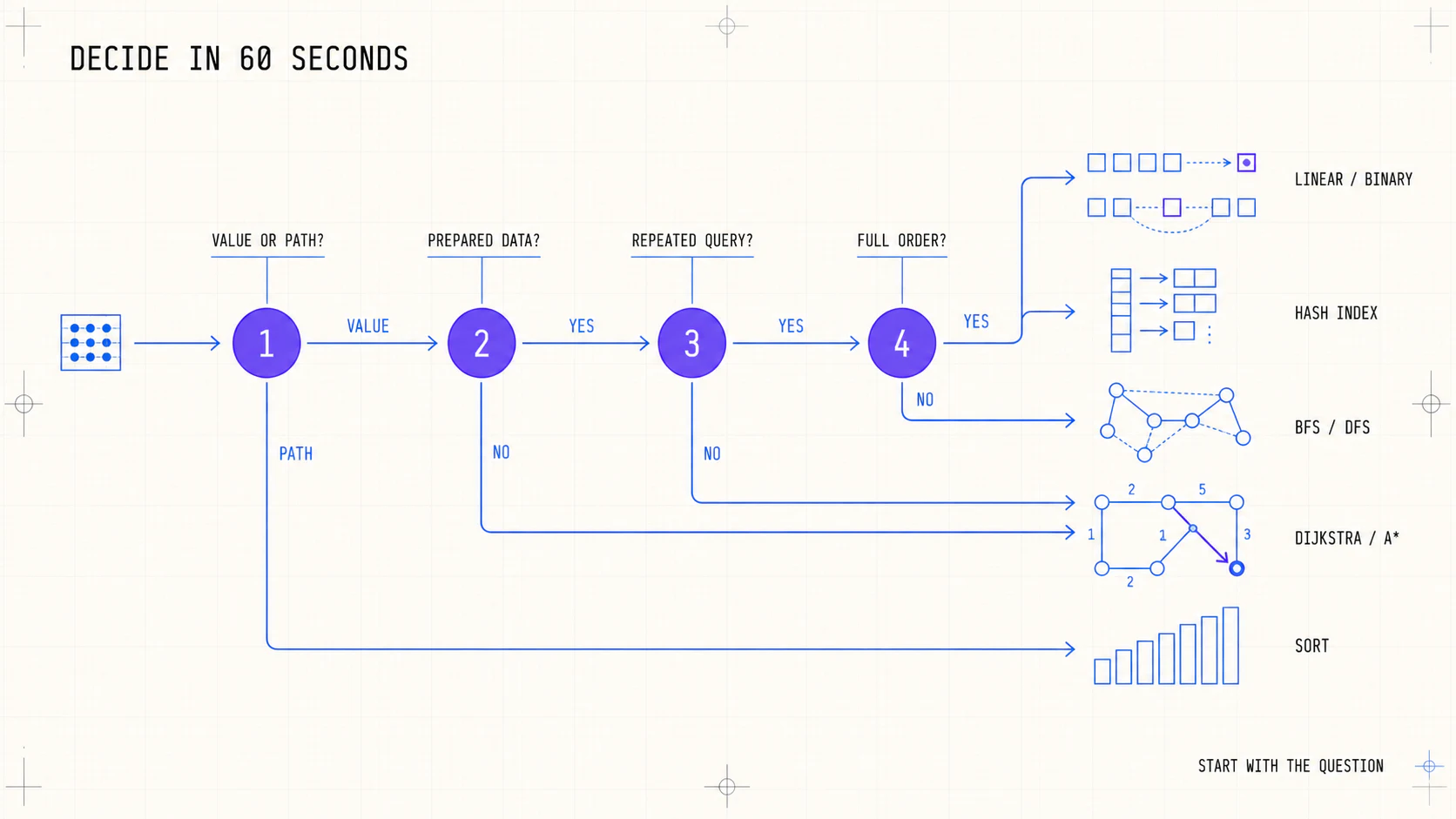 Decision map across search, indexes, graphs, pathfinding, and sorting
| Need | Condition | First option | Example |
|---|---|---|---|
| find one item once | unprepared collection | linear search | locate an error in a short list |
| repeatedly query by key | unique or stable key | hash map / index | user by email |
| find boundaries or ranges | sorted data | binary search | first price above a value |
| explore relationships | tree or graph | BFS / DFS | dependencies or components |
| minimize steps | unweighted graph | BFS | fewest moves |
| minimize cost | non-negative weights | Dijkstra / A* | route by time or distance |
| present or process in order | full collection | sorting algorithm | ranking or report |
Sorting before a single search is usually unnecessary work. Preparing an index, however, can pay off when the same query runs hundreds of times.
02. Data shape limits the options
An algorithm does not work in a vacuum. The available structure determines which operations are cheap and which require a full scan.
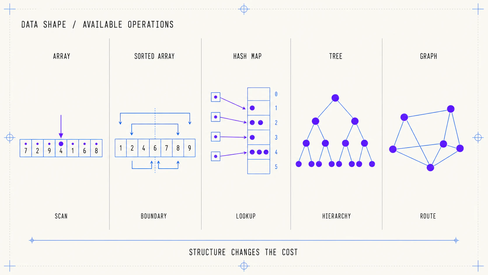 Available operations according to data shape: array, sorted array, hash map, tree, or graph
| Structure | Natural operation | Typical cost | Caution |
|---|---|---|---|
| unsorted array | scan by position | O(n) search | no halving of the search space |
| sorted array | boundaries and ranges | O(log n) search | maintaining order has a cost |
| hash map | lookup by key | average O(1) | no range or neighborhood order |
| tree | traverse a hierarchy | depends on height and shape | may become unbalanced |
| graph | explore relationships and routes | usually depends on V + E | edge weights change the method |
If these structures are not familiar yet, start with Essential Data Structures. To interpret costs without confusing them with milliseconds, read Big O Explained Visually.
03. Prepare once or scan many times
The choice changes when a query stops being occasional. For a collection of size n and q queries, think in terms of total cost:
total cost = preparation + q × cost per query
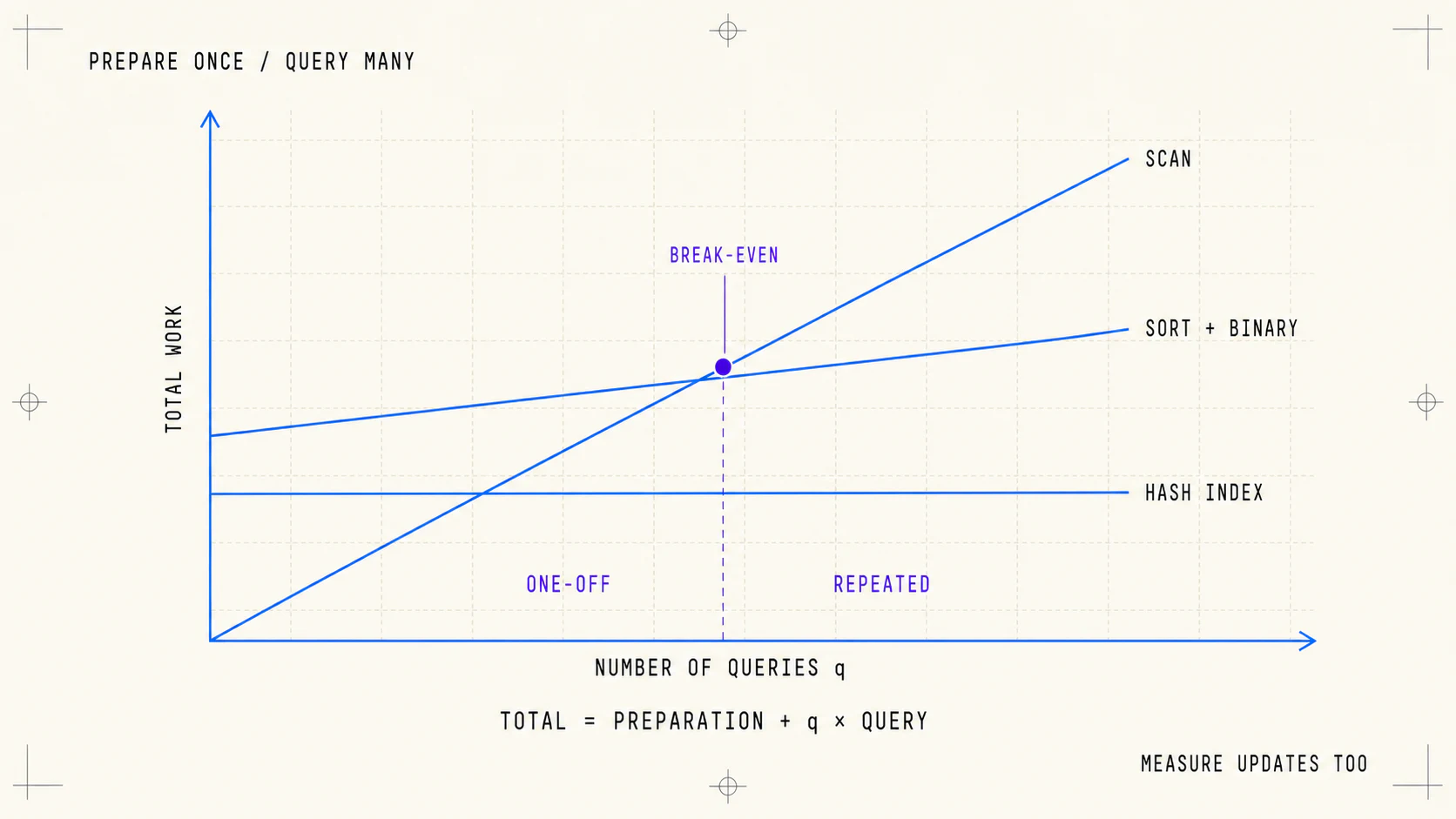 Break-even point between scanning, sorting for binary search, and building a hash index
Linear search has no setup cost, but repeats up to O(n) work per query. An index takes initial time and memory but may reduce each lookup to average O(1). Sorting enables O(log n) binary search, although inserting new data can become more expensive.
| Scenario | Reasonable strategy |
|---|---|
| little data, one query | scan directly |
| many queries by key | build a map |
| many range queries | maintain an ordered structure |
| constantly changing data | measure updates and queries together |
Do not compare only the fastest query. Include memory, update cost, and actual usage frequency.
04. Search branch: value, traversal, or route
Search splits into two main families.
Collections. Linear Search works without preparation; Binary Search requires order; a hash lookup needs a key and auxiliary memory. The choice depends on query volume and whether ranges or ordering also matter.
Graphs and pathfinding. BFS minimizes steps in unweighted graphs; DFS explores depth, components, or backtracking; Dijkstra minimizes cost with non-negative weights; A* uses a heuristic to guide exploration toward a goal.
The Search Algorithms guide develops these decisions. To visually compare the frontier, visited nodes, and reconstructed path, continue with Visual Pathfinding with BFS, Dijkstra, and A*.
05. Sorting branch: the dataset also decides
There is no single winning sorting algorithm for every case.
| Situation | Useful candidate | Reason |
|---|---|---|
| few items or nearly sorted data | Insertion Sort | benefits from short shifts |
| predictable performance and stability | Merge Sort | guarantees O(n log n) |
| strong general in-memory performance | well-implemented Quick Sort | excellent locality; pivot choice matters |
| limited auxiliary memory | Heap Sort | in-place O(n log n) |
| integer keys with a controlled domain | Counting / Radix | exploits key representation |
Bubble and Selection are useful for learning comparisons and swaps, not as default production choices. The Sorting Algorithms guide compares stability, memory, and worst cases. The Canvas 2D visualizer explains how to turn that work into reproducible events and metrics.
06. Recommended route by goal
Use this article as an index, not a destination:
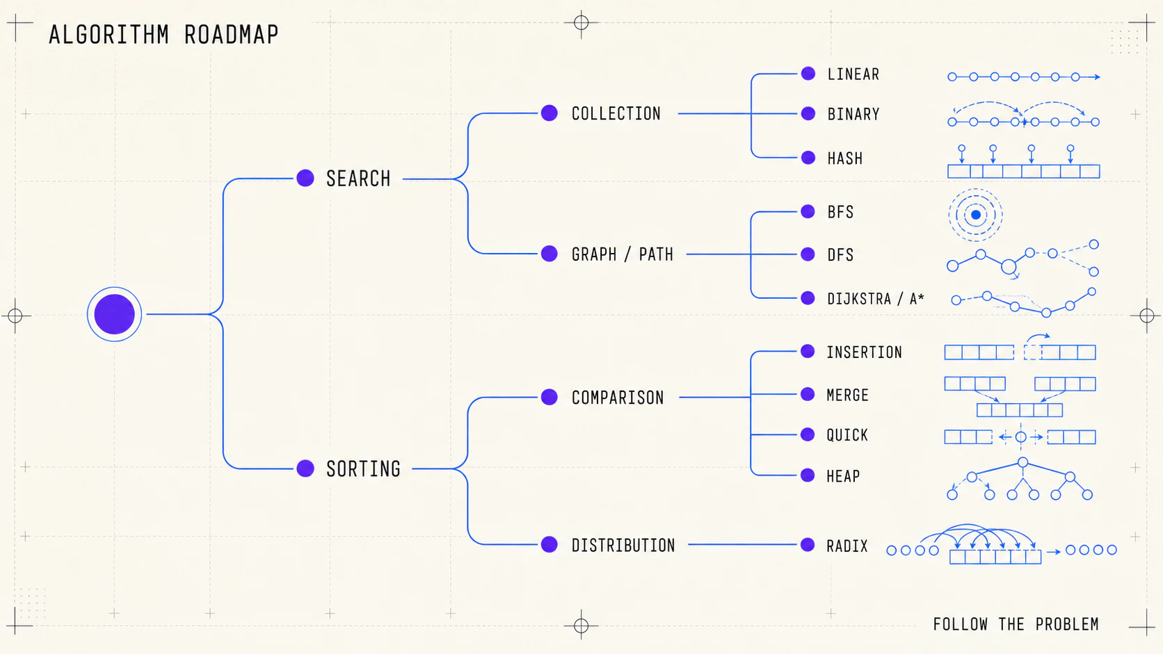 Algorithm family roadmap from search and graphs to comparison or distribution sorting
- Understand growth: Big O and data structures.
- Find a value: Linear Search, Binary Search, and hash indexes.
- Explore relationships: BFS and DFS.
- Find a minimum-cost route: Dijkstra and A*.
- Organize a collection: sorting families and their tradeoffs.
- See the process: visualizers that expose internal state, not only animation.
Before implementing, document the data shape, expected size, query frequency, updates, and the metric you want to optimize. That small brief prevents more wrong decisions than memorizing another complexity table.
The full map becomes: Big O explains growth, structures enable operations, algorithms perform the work, and visualizers make each decision visible.