Sorting Algorithms: How to Choose Between Bubble, Merge, Quick, Heap, and Radix
A practical guide for comparing sorting methods by stability, memory, complexity, data shape, and real-world tradeoffs before choosing one.

Sorting is not only about arranging values. Order can enable binary search, group records, build rankings, or prepare an interface so users can understand the data.
The right decision does not start by memorizing names. It starts with five questions: how large the collection is, how much existing order it has, whether ties must be preserved, how much memory you can use, and what properties the domain provides.
Do not choose the algorithm with the best isolated row; choose the one that preserves the guarantees your product needs.
01. First define what “better” means
Two O(n log n) algorithms can behave differently. One may be stable, another may use less memory, and another may interact better with cache locality. Before comparing names, identify the dominant criterion:
| If you mainly need… | First option to study | Reason |
|---|---|---|
| a small or almost sorted list | Insertion Sort | exploits existing order with little overhead |
| predictable stability | Merge Sort | preserves the relative order of ties |
| strong general in-memory performance | a robust Quick Sort | partitions in place and often has good locality |
O(n log n) worst case with little auxiliary space | Heap Sort | provides a defensive guarantee |
| integers in a small range | Counting Sort | uses the domain instead of comparing every pair |
| keys separable into digits or segments | Radix Sort | processes the key by position |
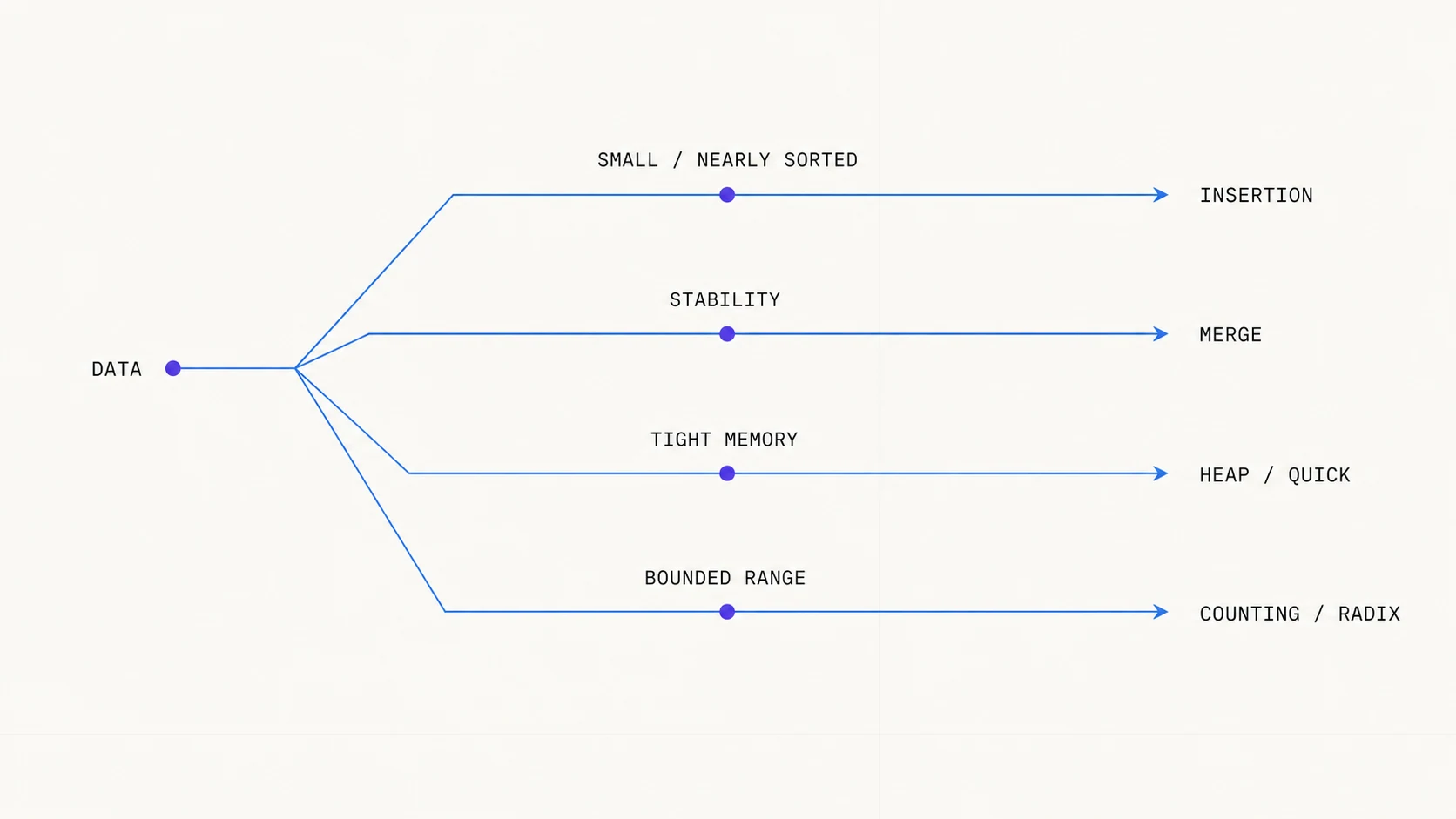 Decision flow for choosing a sorting algorithm from data constraints
Stability means that two records with the same key preserve their relative order. If you first sort people by name and then use a stable method to sort by team, names remain ordered within each team. That guarantee matters in tables, reports, and chained sorts.
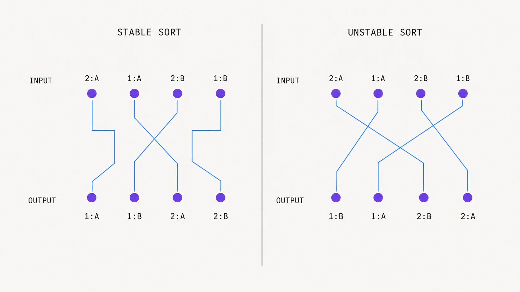 Visual comparison between stable and unstable sorting
It also matters whether an algorithm is adaptive: Insertion Sort approaches O(n) when the list is already almost sorted because it performs few shifts. A non-adaptive algorithm does not automatically gain that advantage.
02. The table you should actually read
Algorithms based only on comparisons have a lower bound: in the general case they need at least Ω(n log n) comparisons. That is why Merge, Quick, and Heap Sort converge around that scale. Counting and Radix can move past it because they use additional information about the domain.
| Method | Best | Average | Worst | Auxiliary space | Stable |
|---|---|---|---|---|---|
| Insertion Sort | O(n) | O(n²) | O(n²) | O(1) | yes |
| Merge Sort | O(n log n) | O(n log n) | O(n log n) | O(n) | yes |
| Quick Sort | O(n log n) | O(n log n) | O(n²) | expected O(log n) recursion | usually no |
| Heap Sort | O(n log n) | O(n log n) | O(n log n) | O(1) | no |
| Counting Sort | O(n + k) | O(n + k) | O(n + k) | O(n + k) when stable | can be |
| Radix Sort | O(d(n + k)) | O(d(n + k)) | O(d(n + k)) | depends on the digit method | yes, with stable passes |
Here, k is the range or number of buckets and d is the number of positions processed. Those parameters prevent us from calling an algorithm “linear” without explaining what its cost depends on.
Big O also does not describe constants, memory access, comparator cost, or allocations. A table gives you the map; a measurement with representative data chooses the route.
03. Simple methods: learn with Bubble, work with Insertion
Bubble, Selection, and Insertion Sort share a quadratic worst case, but they do not offer the same value:
- Bubble Sort makes adjacent swaps visible. It is educational, not a general production choice.
- Selection Sort performs few swaps—at most one per position—but always searches for the next minimum and is usually not stable.
- Insertion Sort shifts an ordered region and benefits from small or almost sorted lists. That is why it appears as a component of hybrid algorithms.
A direct implementation makes its adaptive advantage visible:
function insertionSort(values: number[]) {
  for (let i = 1; i < values.length; i += 1) {
    const current = values[i];
    let j = i - 1;

    while (j >= 0 && values[j] > current) {
      values[j + 1] = values[j];
      j -= 1;
    }

    values[j + 1] = current;
  }

  return values;
}
If every item is already close to its position, the while loop does little work. If the list arrives in reverse order, shifts grow to O(n²).
04. Merge, Quick, and Heap: the same order, different tradeoffs
All three belong to the general O(n log n) world, but they optimize different priorities.
Merge Sort: stability and predictability
It divides, sorts each half, and merges the results. Its running time does not depend on finding a good pivot, and it is naturally stable when ties take the left item first. The usual cost for arrays is an O(n) auxiliary buffer.
It also fits linked lists and external sorting, where the full dataset does not fit in memory and blocks are merged from storage.
Quick Sort: partitioning and strong average behavior
It chooses a pivot, separates smaller and larger values, and repeats on each partition. Its practical advantages come from memory locality and low overhead, not from an absolute guarantee. A systematically bad pivot can produce partitions of 0 and n - 1, taking time to O(n²) and deepening recursion.
Randomizing the pivot, using median-of-three, or switching methods when recursion grows reduces that risk. An industrial implementation is often hybrid; do not assume a language's standard function uses pure Quick Sort.
Heap Sort: a defensive guarantee
It turns the array into a heap and repeatedly extracts the maximum or minimum. It keeps O(n log n) even in the worst case and can work with O(1) auxiliary space. In exchange, it is not stable and commonly has worse memory locality than Quick Sort.
The summary is: Merge for stability, Quick for strong practical average behavior, and Heap when worst-case guarantees and controlled space matter more.
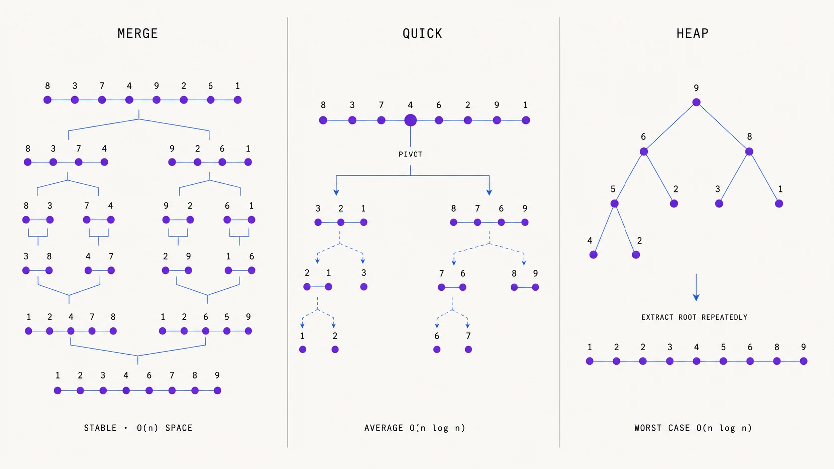 Visual comparison of Merge Sort, Quick Sort, and Heap Sort mechanics
05. When the domain lets you stop comparing
Counting, Radix, and Bucket Sort are not universal replacements. They work because they know something comparison methods do not know.
| Method | Assumption it exploits | Relevant cost | Warning sign |
|---|---|---|---|
| Counting Sort | integer keys between 0 and k | O(n + k) | k is huge compared with n |
| Radix Sort | keys with d positions | O(d(n + k)) | variable digits or an unstable inner pass |
| Bucket Sort | reasonably uniform distribution | average near O(n + k) | one bucket receives almost all values |
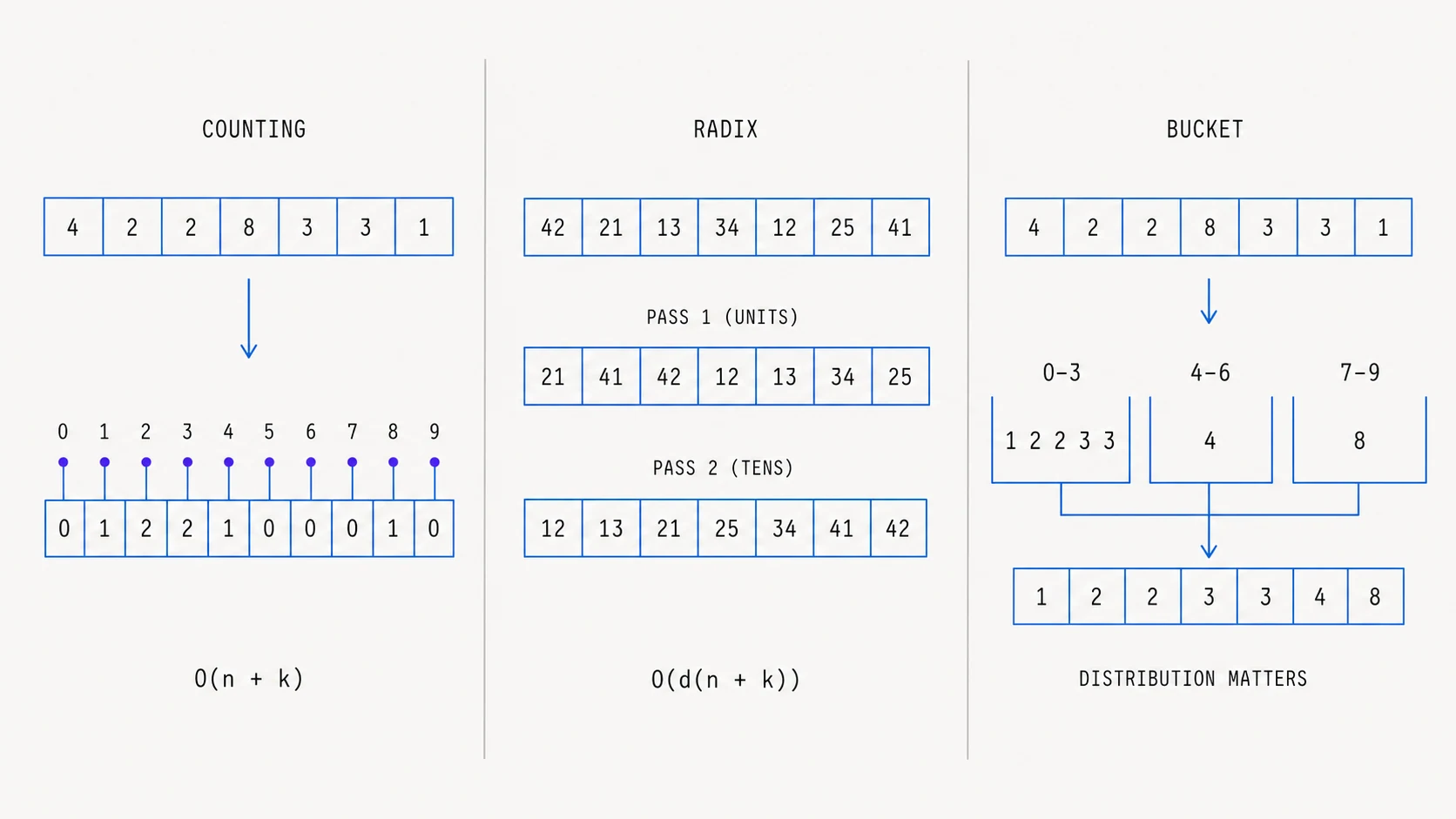 Technical comparison of Counting Sort, Radix Sort, and Bucket Sort
Sorting ten million ages between 0 and 120 is a reasonable Counting Sort scenario. Sorting ten million sparse IDs between 0 and 10¹⁵ is not: the range would destroy the memory advantage.
Radix Sort needs every digit pass to be stable so previous work is preserved. Bucket Sort also needs a strategy for sorting inside each bucket; its performance depends on distribution, not only item count.
06. Practical choice and JavaScript reality
In a product, start with the language's standard implementation. It is usually tested, optimized, and able to combine strategies based on input size or shape. Change approaches when a guarantee or measurement justifies it.
In modern JavaScript:
const users = [
  { name: "Ana", score: 20 },
  { name: "Luis", score: 10 },
  { name: "Mara", score: 20 },
];

const ranked = users.toSorted((a, b) => b.score - a.score);
sort() mutates the original array; toSorted() returns a copy. Both need a comparator to sort numbers or objects with the intended meaning. The standard sort is stable, so Ana remains before Mara when they share a score.
Before implementing your own algorithm, answer:
- Is the collection small, large, or almost sorted?
- Must ties preserve their order?
- Do average time, worst case, or memory matter most?
- Does the domain expose a useful range or format?
- Do you sort once or repeat it on a critical path?
- Do representative inputs confirm the expected advantage?
For learning, implement Insertion, Merge, and Quick Sort. For production, start with the standard tool and measure. For special constraints, choose the family whose guarantee matches the problem—not the one with the most sophisticated name.